Decadal sink-source shifts of forest aboveground carbon since 1988

Reconstruction of global forest AGC

We categorize remotely sensed vegetation variables and environmental data into dynamic (time-varying) and static (time-averaged or time-independent) predictors of AGC (see “Methods”; Supplementary Fig. 1 and Supplementary Table 1). Dynamic predictors include growing-season statistics of CXKu-band VOD, normalized difference vegetation index (NDVI), and leaf area index (LAI), as well as plant functional types (PFTs) of trees and forest cover fractions derived from land cover data. Static predictors comprise aggregated L-band VOD, photosynthetically active radiation (PAR), land surface elevation, and geographic coordinates, which help represent broad spatial and biome-specific heterogeneity¹⁹.

Using a probabilistic deep learning framework based on convolutional neural networks (CNNs)^19,20, we model the spatial relationships between these predictors and the ESA CCI AGC reference maps⁸ (see “Methods”; Supplementary Fig. 1). To improve training robustness, our CNN explicitly incorporates per-grid-cell uncertainty from the ESA CCI AGC products into its loss function, enabling the model to weight observations based on their confidence. Furthermore, to reduce the risk of overfitting to spatial patterns and learning spurious year-to-year fluctuations inherent in individual ESA CCI AGC snapshots (Supplementary Fig. 2), we train independent CNNs for each available reference year (2015–2020) and combine them into an ensemble. This ensemble strategy, together with uncertainty quantification techniques^21,22, yields AGC intervals rather than only deterministic estimates. These intervals represent uncertainties arising from both the inherent noise in the satellite data (aleatoric uncertainty) and the limitations of the model itself (epistemic uncertainty). Finally, we apply the trained ensemble to reconstruct a continuous, harmonized time series of global AGC maps from 1988 to 2021.

We investigate the contributions of predictors to the CNNs’ predictions using an Explainable AI (XAI) approach. Specifically, we aggregate feature attributions based on integrated gradients²³ across CNN ensemble members to quantify predictor importance (Supplementary Fig. 3). This analysis reveals that dynamic predictors account for approximately 56% of total attribution, indicating that time-varying vegetation signals play a major role in the reconstruction. Static biophysical and environmental variables (including PAR, elevation, and L-band VOD) contribute about 26%, leaving static encoded geographic coordinates ( < 19%) to serve as a complementary spatial context for these dominant eco-physiological drivers.

To evaluate its predictive performance, we benchmark our model against conventional empirical VOD-to-AGC conversions and classical machine learning methods (Table 1). While VOD is a valuable biomass proxy, empirical models relying on VOD alone exhibit limited predictive capability on held-out ESA CCI test data from 2010 and 2021 (R² ≈ 0.2–0.6), and their estimated time series of global annual total AGC show weak correlation with the independent 2000–2019 reference records²⁴ (r = 0.35,  p = 0.13). In contrast, integrating multi-source data via our probabilistic CNNs improves both predictive performance (R²= 0.97) and agreement of the global total AGC time series (r = 0.70,  p < 0.001). Compared with classical machine-learning models using the same multi-source predictors, linear models (Lasso and ridge) perform worse in both space and time, whereas random forest achieves comparable predictive performance (R² = 0.98) but lower temporal consistency (r = 0.45,  p < 0.05).

We further compare the reconstructed AGC maps with multiple independent remotely sensed AGC references (Supplementary Table 2 and Supplementary Note 1). Globally, our reconstructions demonstrate strong spatiotemporal agreement with the AGC references, with grid-cell-wise spatial correlations up to 0.87 and temporal correlations of regionally aggregated AGC stocks up to 0.70 (Table 2 and Supplementary Fig. 4). Although this spatial agreement decreases when evaluated within individual biomes, and temporal agreement drops for interannual AGC fluxes compared to total stocks, cross-comparisons reveal even more pronounced discrepancies among the reference datasets themselves due to differing data sources and methodologies (Supplementary Figs. 5–8). Notably, compared to these reference products, our AGC estimates tend to correlate more strongly with each individual dataset than these datasets correlate with each other. This indicates that our observational AGC record provides a useful, internally consistent benchmark for long-term AGC assessments.

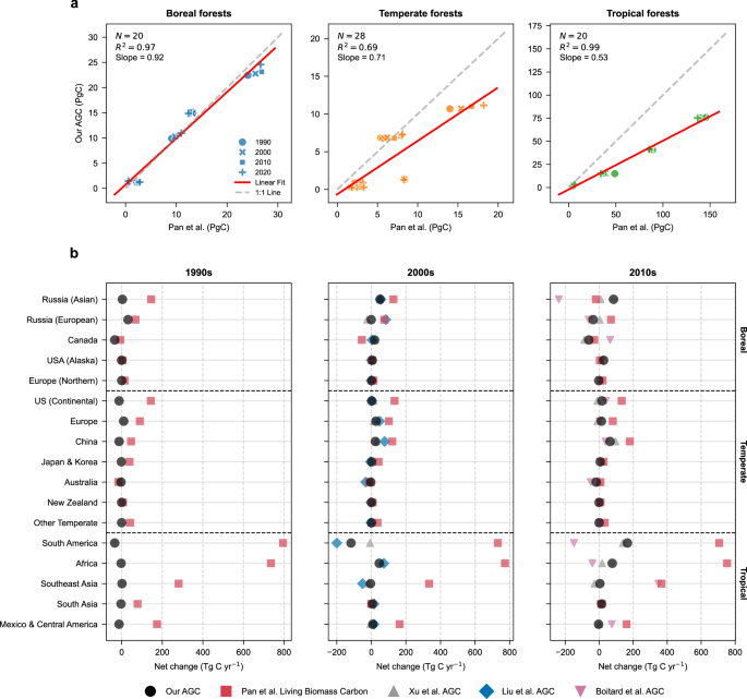
Beyond comparisons with satellite-derived AGC references, we compare our reconstruction with national inventory data of living biomass carbon (i.e., AGC plus belowground carbon) from Pan et al.². Following their biome definitions and temporal intervals (used here only for benchmarking), we find high agreement in regional carbon stocks (Fig. 1a). When evaluating net changes in carbon stocks at decadal scales (Fig. 1b), our estimates generally fall within the spread of values reported by other independent satellite-derived products for the 2000s and 2010s. Furthermore, across boreal and temperate regions, the temporal trajectories of our estimated carbon changes generally align with the inventory-based estimates from Pan et al.². We note that the estimated magnitudes from our model, as well as those from other satellite-derived products, tend to be lower than the inventory data. This discrepancy likely arises from differences in the target variables: assessments by Pan et al.² consider total living biomass carbon, while ours focuses on AGC. Larger discrepancies between satellite-based estimates and inventory data occur primarily in tropical regions. One likely reason is that ground-based inventory coverage is sparse in the tropics, so inventory assessments rely more heavily on bookkeeping approaches to represent losses associated with deforestation and degradation¹⁶. In this context, the contrast between satellite observations and inventories underscores the value of our continuous long-term AGC record as a complement to sparse ground monitoring networks, particularly during the observationally limited 1990s.

a Scatter plots comparing our regional AGC stocks against the living biomass carbon stocks reported by Pan et al.² across boreal, temperate, and tropical forests. Each data point represents a specific geographic region or country for a given year (1990, 2000, 2010, or 2020), following the definitions in Pan et al.². Solid red lines indicate the linear fits, and dashed gray lines represent the 1:1 relationships. The consistent slopes of  < 1 reflect the fundamental distinction between our estimator (AGC only) and Pan et al.’s estimator (total living biomass carbon, which includes below-ground components). b Comparison of decadal net carbon stock changes across regions for the periods 1990s (1990–1999), 2000s (2000–2009), and 2010s (2010–2019). Our AGC change estimates (black circles) are compared alongside inventory-based living biomass changes (red squares) by Pan et al.² and other available remote sensing-based AGC products (Xu et al.²⁴, Liu et al.¹², and Boitard et al.²⁶). Regions are vertically grouped by their corresponding dominant biomes following the definitions in Pan et al.².

Spatiotemporal dynamics of AGC stocks and fluxes

We use our reconstruction to characterize the global distribution and long-term dynamics of forest AGC. Spatially, our estimates reveal high AGC densities in equatorial forests that decline progressively toward higher latitudes (Fig. 2a, c), consistent with independent references^{8,9,10,12,25,26}. The uncertainty (i.e., the standard deviation representing both data uncertainty and the model uncertainties captured by year-to-year variability; see Methods) is similarly elevated in dense tropical forests (Fig. 2b), possibly reflecting higher observational noise and lower predictive skill of CNNs in these areas. Conversely, the relative uncertainty, defined as the ratio of the estimated uncertainty to the estimated AGC, is higher in low-biomass regions; even small deviations in estimated AGC in these areas can lead to disproportionately high relative uncertainty ratios (Supplementary Fig. 9). Categorizing these long-term averages reveals that moist tropical forests dominate global stocks (119 PgC, 52%; median 113 MgC ha⁻¹), followed by temperate (52 PgC, 23%; median 37 MgC ha⁻¹), dry tropical and subtropical (35 PgC, 15%; median 18 MgC ha⁻¹), and boreal forests (24 PgC, 11%; median 17 MgC ha⁻¹) (Fig. 2d, e).

a Multi-year averaged forest AGC density at 0.25^∘ resolution, calculated from the long-term (1988–2021) time series reconstructed in this study. b Multi-year averaged predictive uncertainty (standard deviation), which jointly reflects observation noise and model underrepresentation (see “Methods”). c Latitudinal profiles of zonal AGC stock sums. Profiles represent multi-year means for each reference dataset, except for ESA CCI AGC, which is averaged over 2010 and 2021 to exclude our model training period. d Total AGC stocks of different biomes, with moist tropical forests dominating (119 PgC, 52%), followed by temperate (52 PgC, 23%), dry tropical & subtropical (35 PgC, 15%), and boreal (24 PgC, 11%) forests. e Boxplots of biome-specific AGC density at the grid-cell level, exhibiting a similar cross-biome gradient to the total stocks. The boxplot boundaries from top to bottom represent the maximum, third quartile, median, first quartile, and minimum, and black triangles mark the mean.

Over the period 1988–2021, grid-cell-wise AGC densities exhibit an overall increasing trend (median 0.07 MgC ha⁻¹ yr⁻¹), driven primarily by temperate and boreal forests, while moist tropical forests experienced an overall carbon loss with a median trend of  − 0.04 MgC ha⁻¹ yr⁻¹ (Fig. 3a, e and Fig. 4a). In total, our AGC reconstruction shows that global forests sequestered a net 6.20 PgC in 1988–2021 (Fig. 3f). However, this overall carbon gain masks regional differences (Fig. 4e and Supplementary Table 3). Specifically, temperate forests contributed 3.10 PgC (the largest share of the overall gain), followed by 1.96 PgC from dry tropical & subtropical, and 1.25 PgC from boreal forests, whereas moist tropical forests acted as a weak source of − 0.11 PgC. The widespread AGC sequestration is likely driven by elevated atmospheric CO₂ and, to some extent, nitrogen deposition^27,28. Conversely, deforestation, degradation, and climate change may counteract such benefits in the moist tropics^14,29,30,31.

a Overall AGC density trends across the entire study period at 0.25^∘ resolution. b–d Decadal AGC density trends for the periods 1988–2000 (b), 2001–2010 (c), and 2011–2021 (d). Grid-cell-wise trends are computed via the Theil-Sen slope and a modified Mann-Kendall test to account for serial autocorrelation, with increases shown in blue and declines in red, retaining only grid cells with p < 0.05. e Boxplots of AGC density trends for the globe (gray) as well as moist tropical (green), dry tropical & subtropical (brown), temperate (orange), and boreal (blue) forests. Each box denotes the median, quartiles, and range; black triangles indicate mean values. f Time series of AGC stock changes with respect to 1988 at both global and biome levels, revealing overall increasing AGC stocks in global, temperate, boreal, and dry tropical & subtropical forests, and slightly decreasing AGC in moist tropical forests. Only grid cells with valid data across all years are considered. Shaded areas depict the 95% uncertainty interval (see “Methods”). The vertical gray band denotes the time period affected by the Mt. Pinatubo eruption (1991-1992), which is not included in the time series analysis.

a Annual mean values of net AGC change over the full 1988–2021 period at 0.25^∘ resolution. b–d Annual mean values of net AGC changes for 1988–2000, 2001–2010, and 2011–2021, respectively. Positive changes (blue) indicate net AGC gains, whereas negative changes (brown) denote net AGC losses. e–h Global and biome-specific net changes and trends in AGC stocks for the corresponding time periods. Net changes represent the annual mean AGC difference over each period, while trends are derived from Theil-Sen slope estimates of the AGC stock time series over the same corresponding period. For trend calculation, we consider only grid cells with valid data across all years, and AGC stock values for 1991 and 1992 are ignored. Error bars indicate the 95% uncertainty range (see “Methods”).

We observe a substantial decrease in AGC during 1991 ( − 3.16 PgC), with 92% of this decrease occurring in tropical and subtropical biomes ( − 2.92 PgC). Two major factors may have contributed to this decrease: (i) the compound climate stresses caused by the El Niño/Southern Oscillation (ENSO) and the Mount Pinatubo eruption, as well as the reduction in photosynthetically available radiation after the eruption, which could have caused widespread vegetation mortality^32,33,34, and (ii) volcanic aerosols interfering with remote-sensing data, potentially introducing systematic biases into AGC retrievals³⁵.

Investigating our AGC fluxes for decadal intervals (i.e., 1988–2000, 2001–2010, and 2011–2021) reveals pronounced temporal variability, probably driven by episodic climate extremes and shifting anthropogenic pressures (Figs. 3b–d, 4b–d, and Supplementary Table 3). We quantify these dynamics using two complementary metrics: (i) the net change (i.e., sink or source) computed as the difference between the last and the first year of a decade^24,30, and (ii) linear stock trends derived from the Theil-Sen estimator (“Methods”). The reliability of these metrics is supported by Signal-to-Noise Ratio (SNR) evaluations and Monte Carlo-derived uncertainty ranges (Supplementary Figs. 10 and 11 and Supplementary Tables 3, 4). Although grid-cell-level flux estimates are inherently susceptible to high-frequency natural variability, our SNR analysis shows that spatial aggregation at regional and global scales averages out such local noise, yielding robust decadal assessments.

Overall, global forests have remained a carbon sink: Decadal changes are 210.1 TgC yr⁻¹ during 1988–2000, 43.0 TgC yr⁻¹ during 2001–2010, and 196.3 TgC yr⁻¹ during 2011–2021, with positive values indicating carbon uptake by forests. Concurrently, decadal stock trends have continuously increased, with estimated rates of 105.5, 125.5, 265.9 TgC yr⁻¹ for the three respective periods, further confirming the enduring and even strengthening AGC sink of global forests. However, these global trends mask pronounced decadal sink-to-source shifts in moist tropical and boreal forests (Fig. 4 and Supplementary Table 3).

Moist tropical forests acted as a substantial carbon sink (90.2 TgC yr⁻¹) during 1988–2000, but turned into a carbon source (− 190.6 TgC yr⁻¹) during 2001–2010. This transition coincided with a period marked by repeated extreme events, such as droughts^36,37 and fires³⁸, as well as accelerated deforestation prior to 2004³⁹, which has likely contributed substantially to the observed carbon losses. Similar sink-to-source shifts were also observed during 2001–2010 in countries with extensive moist tropical forests, including Brazil, Indonesia, and Peru (Supplementary Table 3). In the following decade (2011–2021), moist tropical forests transitioned toward a weak carbon source according to our dataset ( − 4.7 TgC yr⁻¹). This partial recovery is likely due to reductions in deforestation rates⁴⁰ and regrowth in previously cleared or degraded areas⁴¹, although the specific causal drivers of AGC change remain to be further investigated.

Boreal forests transitioned from a carbon sink (9.9 TgC yr⁻¹ and 85.8 TgC yr⁻¹ in the first two decades from 1988 to 2010) to a weak carbon source ( − 2.5TgC yr⁻¹) in 2011–2021 (Supplementary Table 3). Growing disturbance pressures, including fire, insect outbreaks, and logging⁷ may have contributed to these substantial AGC losses. Spatial patterns highlight marked declines across parts of eastern Eurasian boreal zones (Fig. 4), while some areas, such as western Siberia, show signs of recovery in 2011–2021 (Supplementary Table 3). Canada’s boreal forests exhibited strong decadal variability, alternating between source and sink over the three decades covered by our dataset (Supplementary Table 3), likely reflecting natural variability, possibly in combination with the influence of regional disturbances⁴².

While temperate forests sequestered an average of 94.0 TgC yr⁻¹ and dry tropical & subtropical forests stored about 59.2 TgC yr⁻¹ over 1988–2021, regions such as Europe and Australia show sink-to-source shifts accompanied by high net AGC losses. In Europe, forests have transitioned to a weak source of  − 10.5 TgC yr⁻¹ in the last decade, when regarding the net AGC change, despite retaining a small positive stock trend of 2.6 TgC yr⁻¹. Previous studies attributed these losses to climate-related storms, pests (e.g., bark beetles), droughts, and fires⁴³. Australian forests remained a net carbon source over the full period since 1988 ( − 2.5 TgC yr⁻¹ on average), as short-term recovery was offset by major drought and fire events, particularly in 2019–2020⁴⁴.

Beyond these decadal sink-source shifts, we analyze interannual variability in AGC fluxes to identify which biomes drive year-to-year fluctuations in global forest AGC. We adopt the flux partitioning approach developed by Ahlström et al.⁴⁵, which considers both the magnitude and the correlation of regional flux anomalies relative to the global signal. We note that these estimates reflect variations solely in the AGC pool; total land-atmosphere carbon fluxes are additionally influenced by variability in belowground and soil carbon pools, which are not captured here. We estimate that dry tropical and subtropical forests contributed 37% of the interannual variability in global AGC fluxes over the past 30 years (1989–2021), followed by moist tropical forests (25%), boreal forests (23%), and temperate forests (15%) (Supplementary Fig. 12). These fractions indicate that dry tropical & subtropical terrestrial forest ecosystems are major drivers of the global interannual variability, consistent with earlier findings⁴⁵, and potentially linked to the vulnerability of these ecosystems to climatic impacts. However, these contributions have changed over recent decades (Supplementary Fig. 12). Temperate and boreal forests collectively dominate in the first (1989–2000) and third decade (2011–2021), accounting for 71% and 90% of the variability, respectively. In contrast, during the second decade (2001–2010), moist tropical and dry tropical & subtropical forests take the lead, contributing 86%. These temporal shifts may reflect changing disturbance regimes across regions. For instance, warming-related stressors and insect outbreaks may have exerted a stronger influence in high-latitude forests during the first and third decade⁷, whereas tropical ecosystems in the second decade appear to have been more strongly affected by deforestation and degradation³¹.

Tropical AGC dynamics

Given that our reconstruction reveals more pronounced decadal variability in tropical AGC compared to other regions (Fig. 4 and Supplementary Table 3), we now focus specifically on the dynamics of these critical ecosystems. To investigate tropical AGC dynamics and their coupling with the global carbon cycle, we analyze the correlation between interannual AGC fluxes and the atmospheric CO₂ growth rate, both linearly detrended over the 1988–2021 period. By computing these correlations across distinct decadal intervals, we observe a strengthening negative relationship over recent decades, reaching r = − 0.63 (p < 0.05) in the most recent decade (Fig. 5a). A 10–year moving–window analysis and uncertainty quantification via bootstrapping corroborate this increasingly negative correlation (Supplementary Fig. 13). These observations may point to a strengthening role for tropical forest AGC in modulating the terrestrial carbon cycle variability.

a Annual AGC flux (black) over pan-tropical forests, spanning approximately 23.5^∘N to 23.5^∘S, compared with atmospheric CO₂ growth rate (blue), both with long-term linear trends removed to highlight interannual variability (IAV). Asterisks (*) indicate statistical significance at p < 0.05, using the two-tailed t test. b IAV contribution of different sub-regions to the overall interannual variability of pan-tropical AGC fluxes across tropical America, Africa, Asia during four time periods (D1: 1989–2000, D2: 2001–2010, D3: 2011–2021, All: 1989–2021). Sub-regions include the Amazon, Congo, and Indonesian rainforests, and the remaining non-rainforest areas. c Time series of AGC stock changes with respect to 1988 for all pan-tropical forests. d–i Corresponding AGC stock changes for tropical America (d), Amazon rainforests (e), tropical Africa (f), Congo rainforests (g), tropical Asia (h), and Indonesian rainforests (i). Only grid cells with valid data across all years are considered. Gray-shaded regions in each panel represent the 95% uncertainty intervals (see “Methods”). Blue-shaded regions represent the uncertainties in CO₂ growth rates. The vertical gray band is the period of the Mt. Pinatubo eruption, not included in the time series analysis. Vertical red shading represents the drought-affected area fraction across tropical forest grid cells, based on the three-month Standardized Precipitation Evapotranspiration Index (SPEI3). Grid cells with SPEI3≤ − 1 are classified as drought-affected.

To understand spatial patterns within the tropics, we assess the relative contributions of different regions to overall AGC variability and examine the heterogeneity of AGC dynamics. Again using the flux partitioning method⁴⁵, we find that the interannual variability in tropical AGC fluxes originates mainly from tropical America and tropical Africa (each contributing  ≈ 46%), whereas tropical Asia accounts for only 7% (see bars labeled ’All’, representing the full period, in Fig. 5b). Within these continents, the Amazon rainforest dominates tropical America’s contribution by accounting for 69% of its interannual variability, followed by the Congo rainforests contributing 24% within tropical Africa, and the Indonesian rainforests contributing 6% within tropical Asia. These patterns underscore Amazon’s pivotal role in shaping tropical AGC dynamics at the interannual scale.

Although tropical forests gained a total of 1.3 PgC from 1988 to 2021, with a trend of 2.7 TgC yr⁻¹, this overall balance masks pronounced regional disparities (Supplementary Table 3). We find that neither tropical American forests overall nor the Amazon rainforest in particular have fully returned to their 2003 AGC levels, although partial recovery occurred after several subsequent AGC losses (Fig. 5d, e). In contrast, AGC in tropical African forests and the Congo rainforest in particular show a relatively stable period between 1998 and 2011, and a substantial decrease in 2015/16. Since then, their AGC trajectories have diverged: Tropical African forests have largely recovered, approaching the 2014 peak, whereas the Congo Basin has remained  ~ 0.3 PgC below its 2014 level (Fig. 5f, g). In tropical Asia, the divergence in AGC dynamics between continental-scale forests and the Indonesian rainforest is particularly pronounced. Tropical Asian forests exhibited an overall upward trend (2.2 TgC yr⁻¹), reaching a peak in 2015 followed by a sharp decline in 2016, with partial recovery in subsequent years that has not returned to the peak level. Meanwhile, the Indonesian rainforests followed a long-term declining trajectory ( − 3.6 TgC yr⁻¹)(Fig. 5h, i and Supplementary Table 3). The continued deforestation and land-use change in the Congo and Indonesian rainforests likely contributed to their divergence from continental AGC trends^46,47.

Previous studies have reported that certain major tropical drought events were associated with substantial carbon losses^48,49. To examine such dynamics in our dataset, we compare regional AGC dynamics with moisture availability conditions quantified as the fraction of grid cells with three-month Standardized Precipitation Evapotranspiration Index (SPEI3) ≤ − 1 ⁵⁰ (see background coloring in Fig. 5c–i). While localized AGC losses co-occur with severe moisture stress during specific events, the broader regional relationship is often less distinct. For example, the Congo and Indonesia rainforests occasionally exhibit sharp declines in AGC without corresponding peaks in drought fraction (Fig. 5g, i). Such mismatches likely reflect confounding influences, including concurrent anthropogenic disturbances and other climate extremes, that also shape AGC dynamics. However, for the Amazon, we specifically examine four well-documented large-scale drought events (1997/98⁵¹, 2004/05⁵², 2009/10³⁷, and 2015/16⁵³) and indeed observe pronounced minima in Amazon AGC stock during the latter three drought years (Fig. 5e). This alignment suggests that climate extremes are driving substantial carbon losses in the Amazon.

AGC loss in the Brazilian Amazon under compound disturbances

The interannual variability in AGC fluxes across tropical forests stems from a complex interplay between human activities, climatic variability, and plant physiological responses⁵⁴. Focusing on the Brazilian Amazon as a hotspot of this variability^55,56, we investigate the drivers of gross AGC losses (defined as the spatiotemporal aggregation of AGC decreases, excluding gains; see “Methods”). To achieve this, we integrate long-term deforestation records from PRODES⁵⁷ with the Intact Forest Landscapes (IFL) dataset⁵⁸. This allows us to distinguish between intact forests and deforested regions (“Methods”). In intact forests, gross AGC losses are likely driven by natural factors (e.g., droughts, fires, storms, and tree mortality) and indirect anthropogenic impacts (e.g., deforestation-induced edge effects and precipitation alterations)^31,59. In contrast, gross AGC losses in deforested regions are more strongly associated with land-use changes, including logging, agricultural expansion, and infrastructure development.

Our partitioning analysis of the interannual variability of gross AGC losses reveals changing contributions from human- and nature-related factors over three decades (Fig. 6). During 1988–2000, AGC losses in deforested areas accounted for 60% of the interannual variability in total gross losses, while intact forests contributed 33%. In the second decade (2001–2010), this balance changed markedly: the contribution of deforested regions dropped to 32%, whereas that of intact forests surged to 59%. This shift might reflect, in part, the influence of stricter deforestation-reduction policies introduced after 2004 (Fig. 6a), which suppressed the variability from direct clearing, alongside severe climate anomalies driving fluctuations in intact forests. In the final decade (2011–2021), although deforestation rates began to increase again after 2012 (Fig. 6a), the average annual deforested area (7681 km² yr⁻¹) remained lower than in the preceding two decades (16,959 km² yr⁻¹ during 1988–2000 and 16,531 km² yr⁻¹ during 2001–2010). Consequently, this persistently lower baseline of direct clearing reduced its influence on year-to-year fluctuations, with deforested areas contributing only 13% to interannual variability. In contrast, intact forests dominated the variability (76%), indicating a growing role of other disturbances, and potential environmental stress induced by anthropogenic climate change on carbon loss in intact forests.

a Time series of annual deforestation area, as reported by the Brazilian National Institute for Space Research (INPE)⁵⁷. b Interannual variability (IAV) of regional AGC gross loss fluxes, partitioned into contributions from deforested regions (orange; Contrib. DF) and intact forests (green; Contrib. IT). The gray shaded band indicates the period affected by the Mt. Pinatubo eruption, which is excluded from the temporal analysis. c Spatial distribution mask of intact forests (green), derived from the Intact Forest Landscapes (IFL) project⁵⁸. d, e Spatial patterns of deforestation fraction aggregated at 0.25^∘ resolution for 1988–2010 (d) and 2011–2021 (e) from INPE PRODES⁵⁷. f–h Spatially explicit patterns of annual AGC gross loss at 0.25^∘ resolution for three decadal intervals: 1988–2000 (f), 2001–2010 (g), and 2011–2021 (h).

Spatially explicit maps of decadal gross AGC losses also corroborate these patterns (Fig. 6f-h). From 1988 to 2000, high gross losses were heavily concentrated along the so-called “Arc of Deforestation” (Fig. 6f), implicating direct human clearing as the principal driver. However, in 2001–2010, this loss footprint expanded extensively across both deforested regions and intact forests, probably reflecting a more widespread effect of disturbances. By 2011–2021, the primary losses occurred in intact forests, and the deforestation arc signature weakens in the gross-loss maps (a pattern also evident in Figs. 3d, 4d). These spatial patterns are closely associated with the evolving spatial distribution of the deforestation fraction (Fig. 6d, e) and align geographically with key degradation drivers identified in previous research³¹.